What is a bandpass filter?
 

Passband of the described interdigital filter, tuned for 426.25 MHz video.  (Vert:  5 db/div, Horiz:  2 Mhz/div)

A Bandpass filter, as the name implies, is a filter that only passes a certain range of frequencies (a spectrum analyzer plot of the interdigital bandpass  filter described below is shown to the left.)  Bandpass filters are the elements that allow any receiver to have selectivity, eliminate image responses, and prevent overloads from off-frequency signals, to name a few examples.  Bandpass filters take many physical forms including capacitors and coils, pieces of feedline, cavities, and waveguides.  The interdigital filter is but one implementation of a bandpass filter.  It is so-called because of the physical construction of filter itself.  Referring to the image below, you can see that the elements are interleaved, and hence the name.

The Interdigital Filter consists of these interleaved rods sandwiched between two parallel conducting plates (ground planes), usually with conductive plates along the sides.  The "height" of the filter (the vertical dimension on the image) is typically one-quarter wavelength while the elements themselves are physically shorter (or else both ends of the rods would touch the walls!)  Because the dimensions of these filters are one quarter of the physical wavelength at the frequency at which they were designed, building such a filter (using air as the dielectric) for frequencies much below the 70cm amateur band would involve a physically large filter.  It is not uncommon to find an interdigital filter for frequencies as high as 8-10 GHz.
 

Pictorial diagram of the described interdigital filter. (Drawing is not to scale)

Why go through the trouble of building such a filter?  Why can't one simply use a pile of coils and capacitors?  At the frequencies involved, the losses and small physical sizes of such components make them difficult to work with and can severely limit their power-handling capabilities.  Why can't one simply use a cavity or two?  Well, you can, but the precise application may dictate something other than a cavity filter.

The response of a single cavity is limited to that of just a single peak (in the area of the fundamental design frequency, that is.)  Its shape can be stretched to a broad peak with gently sloping sides, a narrow spike with fairly steep sides, or anything in between by adjusting coupling and/or Q but you cannot get a broad, flat response with steep sides.

Why would you want a filter that was both wide and sharp?  This sort of filter is invaluable for video, data, and other applications where this is precisely the sort of response that is desired.  To get this type of response, one requires several filter sections.  This could be done with several cavities, but it takes very careful attention to details like coupling and tuning in order to provide a desired response and the resulting filter network will likely be quite large, fragile, and very expensive.

One (of the several) way(s) to get a multi-pole filter that can do what we want is with a properly designed interdigital filter.  We needed such a filter for the transmitter of the WB7FID ATV repeater (a 70cm inband repeater) to attenuate the lower sideband (which was regenerated somewhat by nonlinearities in the amplifier chain) and to keep low-level intermod products from the transmitter out of the receiver.  The picture below shows an example of a filter that we (Clint KA7OEI, Dale WB7FID, and Marv KA7TPH, and Dave, N7UWQ) built several years ago.  It is constructed of 1/8" thick aluminum plate and it is partly TIG welded and partly screwed together.  (The "top" cover and coaxial connectors are really the only components that are held on by screws.)
 

Exterior view of the 7 pole interdigital filter

 Assembling a filter with the desired characteristics isn't trivial, though.  The internal dimensions play a large part in determining the bandwidth, the steepness, the center frequency, and properties of the bandpass (i.e. ripple.)  For design guidance, we have used a program that first appeared starting on page 12 in the January 1985 issue of Ham Radio magazine.  This program was written in BASIC and it can downloaded from here.  (Dale Heatherington, WA4DSY, has an online version of this same program - see the link at the bottom of this page.) In this form, it has been written to run under the old GWBASIC but it should run with minimal modification on more current BASIC implementations.  (Note:  To download this program, you might want to click on the link with the right mouse button and choose the "save link as" option.  Note that although the listing of the program appears in the January 1985 issue of Ham Radio magazine, there is an errata that appears a few months later.  The correction (which has been made to the listing provided) fixes a problem with the plots that the program generates and not with the datum that is produced.

How to run the program

Without having access to the article, the program may be somewhat cryptic, so I'll step through a sample design.  Assuming that you've gotten the program to execute in your BASIC implementation, you might want to follow along.  If you do use GWBASIC, I'd recommend starting it with the following command line:

gwbasic intdig.bas > outfile.txt

This will not only run the program, but it will cause the output of the screen to also be "piped" (output) to a text file (called "outfile.txt" in the example) so that you can review (and/or print) its output later using a text editor.

Let's design a filter for 426.25 MHz ATV.

Since the video goes from 425.0 to 431.0 MHz, our center frequency will be 428 MHz (0.428 GHz.)  We want to pass 6 MHz of video with minimal distortion, so we should really design the filter to be 7 MHz wide (to allow for some fudge factor, as the overlap between theory and practice is sometimes smaller than we'd like...)

Another consideration has to do with how much ripple we wish to allow in our passband.  If we specify 0db ripple, we have also specified a Butterworth filter response.  If we do specify a certain amount of ripple, then the program will design a filter with a Chebychev response.  Which type of response do we want?  A Butterworth response has a nice, smooth passband (ideally) but the passband edges typically aren't as sharp as those of a Chebychev filter design with the same number of elements.  A Chebychev has ripple, but it has the advantage of being sharper than a Butterworth filter of similar complexity.

We'll do a compromise:  We'll specify 0.1db of ripple.  This minor amount of ripple will have a negligible affect the video but, for the same number of filter elements, it results in much sharper skirts than you'd get if you'd specified no ripple at all.

We'll design for 7 elements.  Why 7?  I've run the program, and 7 is a nice number:  It produces a fairly low-loss filter with excellent filter bandpass/bandstop properties, suitable for most transmit applications.  For a receive filter, 5 elements would likely be adequate.

Of course, this filter will be designed to operate in a 50 ohm system.

Note that all dimension are in inches.

First, run the program.  You'll be asked:
# OF ELEMENTS, P-P RIPPLE IN PASSBAND (DB)?

At this point, we'll enter:

7, 0.1

for 7 poles and 0.1 db of ripple.

INPUT FILTER CENTER FREQ. (GHz), BW(MHZ)& LOAD IMPEDANCE ZO?

We enter:

0.428, 7, 50

for 0.428 GHz (428 MHz), 7 MHz wide, and 50 ohms.

The next information it wants is:

INPUT GROUND PLANE SPACING, ROD DIAMETER
& DISTANCE TO CENTER OF FIRST AND LAST ROD?

If you look at the picture of the filter, you'll see the long, narrow dimension of the filter (with the tuning screws.)  The "Ground Plane Spacing" is the inside dimension of the "thickness" of the filter.  Again, from experience, a 2.5 inch space makes for comfortable filter dimensions.  The filter elements are assumed to be round, and we'll use 1/2 inch diameter rods.  The "distance to center of first and last rod" cryptically refers the spacing between the center of each end rod (the ones with the taps on them) and the adjacent inside end wall.  1.5 inches is a good distance for this.  (Remember that that makes the rod 1.25 inches from the wall - we are measuring from the center of the rods.)

So, we enter:

2.5, 0.5, 1.5

for the "thickness," rod diameter, and rod-to-endwall spacing.

The next parameter we are asked for is:

NO. OF FREQU. REJECTION PTS AND STEP SIZE (mhz)?

This has to do with the ASCII plot that the program produces.  You can ask for up to 40 points of data and specify the resolution of those steps.  We'll specify 25 steps at 0.5 MHz spacing, so we'll enter:

25, 0.5

At this point, the program will start spitting out data:

CENTER FREQ.  .428 GHZ
CUTOFF FREQ.  0.4245 (ghz) AND 0.4315 GHZ
RIPPLE BW.  7.000029E-03 GHZ
3 DB BW.   7.476034-03 ghz
FRACTIONAL BW. 1.635521E-02
FILTER Q  57.24961
EST QU    3598.194
LOSS BASED ON THIS QU   .809367 DB
DELAY AT BAND CENTER  249.5265 NANOSECONDS
press any key

At this point, you might want to write this information down (or at least start printing the screen if you didn't start GWBASIC with the output piped to a file.)  Here is an explanation of the data:

• Center Freq.:  Well, that's obvious...
• Cutoff Freq.:  This shows the frequencies at which the filter's attenuation hits 3db (for the Butterworth filter) or the amount of specified ripple (in the case of the Chebychev filter.)  In our case, that's where the attenuation hits 0.1db for the last time.
• Ripple BW:  The ripple bandwidth is related to the the distance between the upper and lower cutoff frequencies (above.)
• Fractional BW:  The 1.635521E-02 really means 0.01635521, or 1.635521% bandwidth.  (The percentage that 7 MHz is of 428 MHz)
• Filter Q:  The equivalent "Q" (Quality Factor) of the filter.  Look this up if you don't already know what it means:-)
• EST QU:  The estimated unloaded Q of the elements.
• Loss based on this QU:  Because the Q relates to filter losses, this is a prediction of the insertion loss of the filter.
• Delay at band center:  How much delay this filter introduces at it's design frequency.

Pressing a key will cause the program to generate an ASCII graph of the predicted filter response, the frequency of the data point, and the calculated insertion loss (rounded off to within 1db) of the filter.

Pressing a key again will give some more data:

QUARTER WAVELENGTH = 6.894159 INCHES
THE LENGTH OF THE INTERIOR ELEMENTS = 6.38665 INCHES
LENGTH OF END ELEMENTS = 6.407211 INCHES
GROUND-PLANE SPACE = 2.5 INCHES
END PLATES 1.5  INCHES FROM C/L OF END ROD
TAP EXTERNAL LINES UP  .3113659 INCHES FROM SHORTED END
LINE IMPEDANCES:  END ROD 108.2183, OTHER 110.9835, EXT. LINES 50 OHM

• The Quarter Wavelength is the internal size of the filter (the vertical dimension of the drawing.)
• The "Interior Elements" are those elements that are not on the ends (the 5 in the middle) while
• The "End Elements" are, well, those on each end.
• The "Ground Plane Space" is that 2.5 inch spacing between the two ground-plane sheets (the covers.)
• The "End Plates 1.5 inches from C/L of end rod" is that 1.5 inch spacing of the C/L (CenterLine) of the end elements to the end plates.
• The next line says that the 50 ohm point is 0.311 inches from the ground end and that they should be tapped there.
• The final line just gives some internal impedances that you may or may or may not be interested in as well as the input/output impedance that you specified.

A word of warning:  The above lengths are those predicted for exact tuning assuming that the predictions were perfect.  The reality is that you'll want to be able to tune the elements slightly to allow for the (inevitable) departures from the predicted parameters.  So, you'll actually want to make the elements a few percent shorter than the predicted lengths and you should be prepared to shorten them even more!
 

Building a filter
 

Another exterior view of the 7 pole interdigital filter

Before you start building, design the filter that you believe you want.  This may sound silly, but I strongly recommend that you try several variations of the filter (number of poles, ripple, ground-plane spacing, etc.) and carefully weigh the resulting properties for each predicted filter (i.e. insertion loss, physical size, etc.)  One thing that you'll immediately notice is that the length of the filter increases dramatically with the increasing ground-plane spacing, but the insertion loss goes down.

What material to use?  Silver-plated brass or copper would provide some of the best performance (i.e. lowest loss) but polished copper (without the silver) will work nearly as well (provided that it is protected from moisture...)  Aluminum would be the second best choice, and brass would be the third.

How does one hold the filter together?  Perhaps one of the most practical ways (although laborious and time-consuming) to assemble such a filter is with screws, with threads drilled and tapped.  For this case, you will need at least one screw per element along the length of the filter (that's 4 screws per element if you count the top and bottom screws and the ones on the back.  Along the sides, you'll need to put screws at intervals no larger than the spacing of the elements - and probably more than that, with at least two screws on the "thickness" part of the side walls.

Closeup of the tapped end-element.  The back of the "N" connector and the setscrew connecting to the element may be seen.

In the case of copper, brass, (or other silver-plated metals) the filter can be (at least partially) soldered together.  Of course, you would never want to solder the filter completely together as you would find it extremely difficult to disassemble should repairs (or modification) be necessary.  For Aluminum, you would probably use screws to assemble the filter and using appropriate amounts of anti-oxidant on mating surfaces to assure continuity.  Of course, it is possible to TIG weld the filter (as we did in the filter shown above) or even use aluminum-capable solder (which is expensive and usually contains cadmium - a toxic heavy metal.)

One of the somewhat unusual aspects of this particular filter is that it uses tapped end-elements (tapped at the point at which they exhibit the designed impedance) rather than the end-fed resonators that are shown in the oft-quoted March, 1968 QST article by Fisher.  This makes for simpler construction.  The picture to the right shows the tap-point for our aluminum filter.  You can see the rear of the chassis-mounted N connector and the conductor that goes through the element at the tap point.  In this case, it is a short piece of #12 copper wire, held in place with a hex-head (allen-type) setscrew.  The connection is coated with anti-oxidant to reduce the effects of electrical connections of dissimilar metals.  This filter was built in 1994 and we have never had any problems with these connections.
 

Interior of the interdigital filter, showing one of the elements TIG welded to the sidewall

The elements themselves are also aluminum, but they could have been brass or copper.  Since we had access to a TIG welder, the elements themselves were first mounted with screws and then tack-welded to the sidewall to assure mechanical strength and a consistent electrical connection.  If we had used copper or brass, we would have just used a stainless-steel screw, the connection would be coated with anti-oxidant, and the wall-end of the element would have been counterbored in concave so that the outside "rim" of the element would be making solid contact and not the center of the element, which could "wobble" about.
 

Closeup showing the tuning screws (with capacitive disk) for one of the elements.

How does one tune the elements?  Firstly, remember that these elements are electrically shorter than 1/4 wavelength.  Secondly, remember that the length of the elements as predicted by the program are the idealized lengths for the desired response.  In other words, if everything were perfect these would be the lengths of the elements for the exact response desired.  Since everything is not perfect, you will have to make the elements slightly shorter than the predicted lengths so that they can be tuned for the desired response.  The amount of this shortening is on the order of a few percent and is rather difficult to predict.  Be prepared to trim the elements slightly after the filter is assembled!  In the case of the filter shown, the elements had to be shortened by over 1/8 of an inch.  A rotary tool (such as a Dremel) and a file was used for this task, as the element could not be removed (remember:  it was welded into place!)  Normally, only tuning screws are used and the proximity of the screw to the end of the element adds just enough capacitance to tune the element down into proper resonance.  In the case of our filter, it was originally designed to operate on the 439.25 MHz ATV frequency but we needed to retune it to 426.25 MHz.  While the screws could tune the filter to frequency, the spacing between the screw and the end of the element was very small.  This could reduce the mechanical stability of the filter's tuning and the small spacing could permit arcing at higher power levels.  Small disks were soldered to the end of the screws in order to increase their surface area and thus the capacitance.  On the outside of the filter, there are jam nuts on the screws (both of which are brass, by the way) to allow the filter tuning to be locked once the desired response is achieved.
 

Full interior view of the interdigital filter.

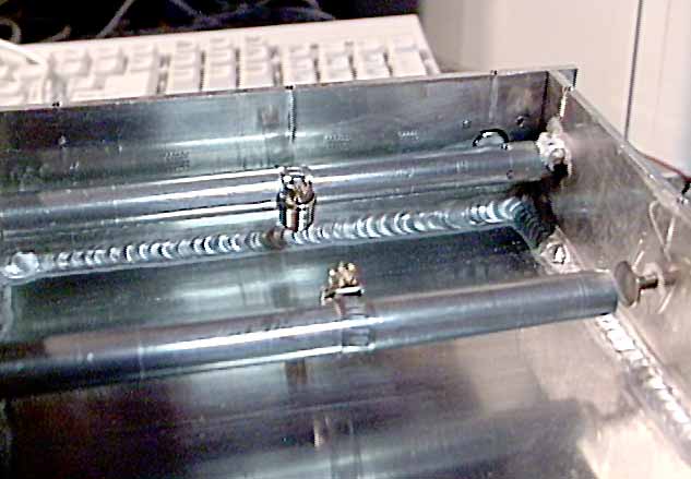
The interior of the complete filter is shown to the left.  Although they are difficult to see in the picture, you can just make out the tapped holes at each element and at several points along the sides.  There are 20 screws (14 for the 7 elements, 3 along each side) that hold the top on the filter.  It should be noted that during the initial tune-up of the filter, it was not possible to get any sort of representative filter response without putting the cover plate(s) on and the screws in.  In other words:  If you need to trim the elements to allow them to be tuned, you will have to put the cover(s) back on and the screws in every time you want to see if you have shortened the elements enough.

Tuning the filter

A bit of advice:  Do not even waste your time trying to tune the filter unless you have some test equipment to tune the filter!   Let me say that again.  Unless you have some test equipment, you are going to pull your hair out trying to tune the filter!  Even if you do have the equipment, it is likely that you will still lose some hair!

There are several equipment lineups that will allow tune-up:

• A sweep generator on the input and a diode detector on the output that goes to an oscilliscope, the X-axis of which is driven from the sweep voltage output of the generator.  This is what was used for the original tune-up of the filter and, assuming that the filter isn't so badly detuned that you can't get enough signal to bias the detector, it works well.  If it is badly detuned, one can take the brute-force approach and transmit into the filter with a handie-talkie and twiddle the tuning screws until you get some output and finally have a starting point.  If you don't have a calibrated sweep generator, then do this trick:
• Couple a bit of energy from the sweep generator into an FM receiver.
• Feed the unsquelched audio output into the Z axis (brightness) input of the oscilloscope that you are using on the diode detector.
• If you are careful, you should be able to see the change in brightness on the trace where the generator sweeps through the frequency to which the radio is tuned.
• Doing this, you can figure out where the start and stop points are on the sweep by tuning the receiver.
• If you have a fast squelch and/or if you use a very slow sweep, you could also squelch the radio and observe the brightness change on the sweep as generator sweeps across the receive frequency and causes an audio "pop" as it breaks the squelch.
• Do this for the "start" and "stop" frequency, noting where they are on the oscillicope.
• What about if you don't have a sweep generator at all?  I suppose you could (carefully!) disconnect the PLL of a synthesized radio and connect the VCO tuning line (with proper voltage scaling and offset) to a sawtooth wave generator (like a 555...)  Assuming you can get the radio to produce output with an unlocked PLL, this makes a dandy, high-powered sweep generator.
• A spectrum analyzer and a tracking generator.  This is handy, if you have it.  It has the advantage that there is a logarithmic display and you therefore have a lot more dynamic range and can see "deeper" into the sides of the response than you can with the diode detector.  If you have access to a spectrum analyzer but not a tracking generator, you can use a broadband noise generator.  (That is how the trace at the top of this page was generated, by the way...)
• You could use a network analyzer.  This is the very best tool for the job, but you may have to ask someone in the RF design industry (or a related field) if they have one and if you can use it...

Plots of the same filter with (left) and without resistive source and termination.  Note that while the filter with the resistive attenuators on the input and output shows about 0.5db of ripple, the one without the pads has almost 2 db of ripple!

If you are using the sweep generator/detector or tracking/noise generator/spectrum analyzer method (or some combination) you must put resistive pads on the input and output of the filter, at the filter!  Even though it may say 50 ohms on the test equipment, do not believe it!  At the very least, the cables will transform the impedance to something other than 50 ohms resistive during the tuning process. Use at least 6 db pads (and preferrably, 10 db pads.)  If you don't do this, you'll be chasing your tail. The two pictures above demostrate this very clearly:  The picture on the left is shown using 10 db pads on both the input and the output while the picture on the right demonstrates the ripple that can result if you rely on the test equipment to source and terminate at 50 ohms (notice the almost 2db ripple on the one on the right!.)  Unfortunately, it can be difficult to maintain a 50 ohm system (using ferrite isolators and watching VSWR helps) but it is important that you have a known starting point. YOU HAVE BEEN WARNED!

Assuming you have the equipment, you are now faced with trying to tune the filter.  It may not be easy to try to tune a filter with numerous highly-interactive adjustments.  If you have a "knack" for such a thing, sometimes you can get the "feel" of the filter by tuning each screw, observing it's effect, and then tuning it by the seat of your pants.  Be forewarned:  Not everyone can do this, so don't kill yourself trying!

The "Dishal" Tuning method:

You must first determine if the elements are short enough (or long enough) so that there is adequate tuning range.  While having a network analyzer is nice, Dale, WB7FID, did some digging through old IRE and IEEE journals and reports that the easiest way to determine what your filter is going to do is with the Dishal method (named after the author of an article where this procedure was described.)  This method requires a signal generator and a slotted line.  The Dishal Method of tuning an interdigital filter is approximately thus:

1. Turn all tuning screws  such that all elements are shorted out on the ends by the tuning screws.
2. Terminate the filter with the proper impedance e.g. 50 ohms (optional, but highly recommended.)
3. Using a fairly high-output signal generator, put a signal into the slotted line on the center design frequency.  Connect the other end of the slotted line to the input of the filter (i.e. the end that is not terminated.)
4. Slide the slotted line to find either a peak or a null of a standing wave. Do not touch the slotted line again during the procedure.
5. Tune the element closest to the slotted line so that the peak becomes a null, or vice versa (depending on what you started with...)
6. Tune the next element for a null or a peak (opposite what the previous element produced...)
7. Repeat the previous step for each of the remaining elements, alternating between the peak and null.

If you have a network analyzer, you can infer from the above procedure what it is that you should be doing.  If the elements are of the proper length, you should be able to easily tune through the null or peak (whatever it was that you tuned for) without the screw being too close to element rod end or being almost completely removed.  In the case of the latter, the element needs to be shortened.  In the case of the former, you cut the element too short and you either need to lengthen it (preferred) or put a disk on the screw.
 

Pictorial of a quick and dirty "slotted line" that may be used to aid in tuning an interdigital filter.

"But I don't have a slotted line.."

If you don't have access to a slotted line, you might want to ask around to find one.  Alternatively, you can construct a "reasonable facsimile" (see the picture to the right.)  This is essentially an open-air transmission line that is suspended above a ground plane.  Ideally, it should be at least 1/2 wavelength long at the test frequency (to allow selection of a peak or a null) but you can make it shorter if you have an assortment of short pieces of coax that you can insert/delete:  The idea is to place the peak (or null) somewhere along the slotted line.  Strictly speaking, this is not really a slotted line, but but the whole point of this exercise is to get access to the center conductor so that you may sample some if its energy.

Place the line (consisting of some brass rod, stiff copper wire, etc.) about 1/8 inch above the ground plane (if you are a purist, you can go ahead and calculate the proper height for 50 ohms...  Since we are utilizing the standing waves anyway, it isn't all that critical.)  With the procedure above (with all elements shorted) you would place the probe very close (but not touching!) to the line and slide the probe (the diodes, etc.) along the ground plane until you find the peak/null.

You may need some reasonable amount of power for this in order to get enough energy to get a good detector reading:  I used a handie-talkie on low power (1/2 watt) for this.  Once you have found the peak/null, you can then tack-solder the ground of the probe to the plane.  Once the ground is soldered down, you can usually move the probe back and forth slightly to fine-tune the peak/null.  Using some circuit board material makes soldering much easier.

For the diodes, use 2835-type shottky mixer diodes, 1N34 types, or 1N914/1N4148 types (in order of most to least sensitive) and all but the 2835 types are available at Radio Shack.  For the capacitor, a small 0.01 uf disk ceramic is adequate.  Keep all leads (except for the probe lead - which could be the lead of one of the diodes) as short as practical.

Alternatively, you could etch (or cut) a 0.110 inch wide line into a length of G10 or FR4 0.062 inch thick double-sided glass epoxy (don't use any other kind!)  circuit board.  Leave about 0.1 inch gaps between the line and the surrounding ground plane.  Wrap the edges of the board with copper foil and drill small holes in the ground planes alongside the strip and put small wires (soldered on both sides) to make sure the ground integrity is maintained.  Like the suspended line, you would place the probe very close to (but not touching) the line.

The results:

This procedure also reveals something about what the "natural" response of the filter is supposed to be.  If you built it exactly right, it will produce a response that somewhat resembles the original design parameters (you hope...)  At this point the tuning should need to be only slightly changed to attain the desired response or, at the very least, you should have a good starting point for tuning.  If you can't get the response that you desire, then there are at least four possibilities:

1. You should try harder, or maybe you should let someone else try:  Maybe they'll have better luck.
2. One (or more) of the elements are too long.  Try tuning it up 5 to 10 MHz lower in frequency.  If it tunes up you need to shorten the elements slightly.  Knowing the frequency at which it does tune up might clue you in as to how much you need to shorten the elements.
3. One (or more) of the elements are too short.  Try tuning it up 5 to 10 MHz higher in frequency.  If it tunes up you need to lengthen the elements (perhaps blobs of solder, in the case of copper or brass elements) or increase tuning screw capacitance (by putting disks on the tuning screws.)  The preferred method is to lengthen the elements.
4. You built the filter wrong!  Hopefully you can figure out what you did.

There are a few things we learned when building our filter (some of which fall under the heading "If we do this again, we'll do this differently!")

• We placed the end elements too close the the end walls.  We believe that this has some effect on the ability to tune the end elements since we had to make them quite a bit shorter than the program suggested.  We also believe that this contributed to insertion loss that was somewhat higher than we predicted.
• Avoid leaving sharp edges on the edges of the elements and tuning screws (or disks.)  The ends should be slightly rounded (we beveled our elements and then sanded the sharpness off.)  If there are sharp points or spikes at the ends of the elements this can lead to flashover if you attempt to run very much transmit power.  Remember that there is high RF voltage at the ends of these elements!
• We used 1/8 inch aluminum plate for the entire filter.  This is plenty thick enough for adequate mechanical stability:  It takes a lot of pressure on the top/bottom to (temporarily) detune the filter and once pressure is released, the original tuning is restored.  The biggest problem is that 1/8 inch thick plate is just not thick enough to comfortably accept drilled and tapped 4-40 screws.  If you look carefully at the picture above that shows the element tack-welded to the sidewall, you'll notice a "bulge" in the sidewall where the threads were drilled and cut.  None of the screws have actually stripped out, fortunately.  To prevent this from happening, there are several possible solutions that occur to me:
• Use thicker metal.
• Use smaller screws.  (This isn't a very good solution in my book...)
• Run a weld bead on the outside and/or inside of the wall to increase the effective thickness where the screw will be.  This would be true for TIG-welded aluminum filters.  For copper/brass, I suppose you could braze more material there...
• Weld/Braze/Solder a piece of metal on the outside of the filter and drill/tap into that, instead.  You could even attach an already-threaded standoff.
• Run very long screws (or use some "allthread") between the top and bottom covers and don't even tap into the filter.  The compression between the two covers should keep the covers in place.
Remember, you still need to figure out how to hold the sides of the filter together (i.e. solder, welding, brazing, or with screws.)
• We would connect the tap-points of the end elements differently so that we could adjust the tap points slightly.  I'm not sure exactly how we would do that with aluminum rods, but we really haven't thought about it much.  With brass/copper rods, the tap-points could be soldered into place.
• A word of warning:  This filter is based on 1/4 wavelength elements.  Like any filter with elements that are based on odd 1/4 wavelength elements (this includes cavity filters!) it will have a bandpass response at odd multiples of the 1/4 wavelength frequency!  In other words, almost any 70cm interdigital, combline, or cavity-based filter will pass some 23cm signal through it.  The response and insertion loss may be poor, but signals will get through!  If you are running a crossband repeater with a 70cm transmit at a 23cm receive, your 3rd harmonic may cause you some grief.  You will want to place a lowpass filter somewhere in the line (after the isolator/circulator, if you have one, as it can generate harmonics and intermod of its own, plus it doesn't work well too far from it's design frequency!) to prevent this energy from getting through.  We will be using a disk-and-rod filter that was extricated from a commercial 450 Mhz transmitter, but you could use practically anything.
• I should mention that the design parameters given above reflect more along the lines of what we should have done, and not what we did do.  For example, the end elements are too close to the side wall.

• Insertion loss at 439.25 Mhz:  1.3db
• Insertion loss at 442.83 (Chroma subcarrier):  2.1 db
• Measured 3db bandwidth:  about 7.5 MHz

When we did the final tuneup we were fortunate enough to have access to an HP Network Analyzer.  After "diddling" the tuning for a while, we noticed that we could get the tuning absolutely flat if we wanted an insertion loss of about 1.8 db or so, or we could tune it to favor the video carrier frequency and cut our losses by about 0.5 db.  We chose the latter since that is where most of the power is:  We could always crank up the chroma a bit on the video processor (and we did) to make up the difference.  I don't remember what the group delay parameters were precisely on the final tuneup, but they were more than acceptable for amateur use (the effects weren't visible in the video, anyway.)

When we recently retuned the filter for the 426.25 MHz video frequency (remember that this filter was designed for 439.25 MHz!) we got approximately the following results:

• Insertion loss across the passband:  2.3 db
• Ripple:  <0.5 db
• 3 db bandwidth:  6.8 MHz
• 10db bandwidth:  8 MHz
• 20 db bandwidth:  10 MHz
• 30 db bandwidth:  12 MHz
• 60 db bandwidth:  19 MHz
• 80 db bandwidth:  32 MHz
• 110 db bandwidth:  43 MHz

The spectrum analyzer plots above (the one at the top of the article, plus the two showing the effects of not providing proper resistive termination of the filter) are of this filter, as tuned for the 426.25 MHz frequency (the filter center frequency is 428 MHz, 5 db/vert. div., 2 MHz/horiz. div.)

You'll have noticed two things here:  The insertion loss was higher, and the filter was tuned for flatness and not for "minimum attenuation where it matters most."  The increased insertion loss is likely the result of the taps being in the wrong positions for the frequency, and for the internal dimensions of the filter being a bit too small.  Additionally, we had to put the disks on the tuning screws in order to load the resonators down to the proper frequency and that probably increases the losses slightly.

Update (1/16/2000):

Dale, WB7FID, has been working on integrating the various components of the repeater.  We have both been somewhat disappointed by the performance of the filter and have been determining ways to fix it, or mitigate its problems.

The apparent "lossiness" of this (or any) filter can be attributed to several things (this is not an exhaustive list):

1. Resistive losses.  Electrical resistance is the ultimate show-stopper in the persuit of the "ideal" filter (i.e. lossless, perfect response, etc.)
2. Mismatching.  If you throw 10 watts into a filter and it throws 5 watts back at you because of mismatch, then it doesn't matter whether or not the filter is intrinsically lossy or loss-less.

What might cause the apparent mismatch?  Here are some possibilities:

• Mis-adjusted tap points on the elements. (the filter uses tapped end elements which, unfortunately, cannot be adjusted...)
• Under or Over-coupled filter elements.
• Mistuned filter.

Modified 7 element interdigital filter showing the hoseclamps to increase coupling

Dale, who works at a local (to him) University (in a microwave/RF-type lab, as it turns out) has access to a network analyzer which allows him to do definitive "before" and "after" comparisons.  The first item of business was to find the "natural" response of the filter using the dishal method (described above.)  In very general terms, if the filter is too narrow, it is undercoupled.  If it is too wide, it is overcoupled.  In our case, Dale found that the filter was about 6 MHz wide - and our target was a bit over 7 MHz wide.

How does one increase coupling?  One obvious solution is to move the elements closer together.  Equally obvious was the fact that we weren't going to be able to do this with the already-built (and welded) filter.  Another way to increase coupling is to increase the diameter of the rods themselves.  That wasn't much of an option, either, as the elements themselves are aluminum (we didn't want to try welding more metal onto them because we didn't know how much...)  The obvious solution (to us) was to put some very small hose clamps on the elements:  This will increase the apparent diameter of the element, and (importantly) the amount of coupling is variable by the virtue of the fact that the elements may be moved about, and that a greater (or lesser) number of clamps may be added as needed.
 

Network Analyzer plot of final tuning.  (Click on image for full-sized view)
Before and After summary:
At the video carrier frequency insertion loss dropped from 2.3 db to about 1.8 db!

The picture shows two clamps in the center of one of the end (tapped) elements and its adjacent element.  Dale did some extensive experimentation (with more and fewer clamps) and found that the above combination worked very well for this filter.

A note:  Placing the clamps near the ground end of the elements will have less coupling effect from that element while placing it at the open (high impedance) end will possibly couple more energy, but it will also significantly change tuning (as the end of the element is effectively bigger) and, if high power is being used, the sharp edges of the clamp may allow corona or arcing to occur.  We chose to put our "coupling clamps" in the middle of the elements.

The result?  Look at the chart on the right!  (and click on it to get a bigger view.)  You'll notice that the insertion loss at the Chroma and Sound frequencies (which also pass through the filter) is higher, but since they represent only a small percentage of the total energy, the additional losses incurred may be compensated by increasing the chroma output of the video processor (if you have one) and the aural transmitter power (we use a completely separate audio transmitter as described here.)  The return loss isn't a whole lot better than it was, but we are either going to:

1. Ignore it (we are using ferrite isolators to absorb reflected power) or
2. Try a tuning device such as a 2-slug tuner on the input/output lines to provide a better match.

Looking forward:

Actually, we are building a new filter.  This one will also be made out of aluminum, but it will have silver-plated copper rods.  It will be much larger (physically) and we are trying to get the insertion losses well under 1db.  It will not be TIG welded together (as the heavier stock makes that more difficult) but rather it will be put together with lots of stainless-steel screws and anti-oxidant to maintain good connections and to prevent the screws from seizing in their threads.  We have just acquired most of the material but, since we already have a useable filter (the old one) we'll go forward with the repeater project and get it on the air with the old filter first:  We'll worry about replacing the filter once we're on the air.

From the WA4DSY site, there is an online calculator on the  Design a custom Interdigital Bandpass Filter page.

Return to the  Utah ATV Home Page or to the  WB7FID Repeater Transmit Filter/Combiner subsystem page.

This is an evolving document so check back occasionally.  If you have any questions or comments, please email them.

This page updated 20030513